Embeddings are a core AI concept that underpin a great deal of what we today think of as being AI. This article is going to give you an accurate and intuitive understanding of what an “embedding” is in less time than it takes to eat a (very large) bagel, and possibly make you think they’re as cool as I think they are. It even explains how we got to embeddings as a solution, by looking at everything else we tried along the way. If you’re comfortable with even very simple Excel formulas, you’ll understand all the maths, and there’s even a cute graph with dogs on it.

Classifying dogs

Let’s start by thinking about dogs, and by classifying them by their attributes:

Breed	Size	Intelligence	Note
Great Dane	5	5	Great Danes are big and clever
Shih Tzu	1	1	Shih Tzu’s are small and not deep thinkers
Border Collie	3	5	A clever boi
Beagle	2	3	Kinda small, kinda smart
Bulldog	3	2	Kinda large, kinda dumb

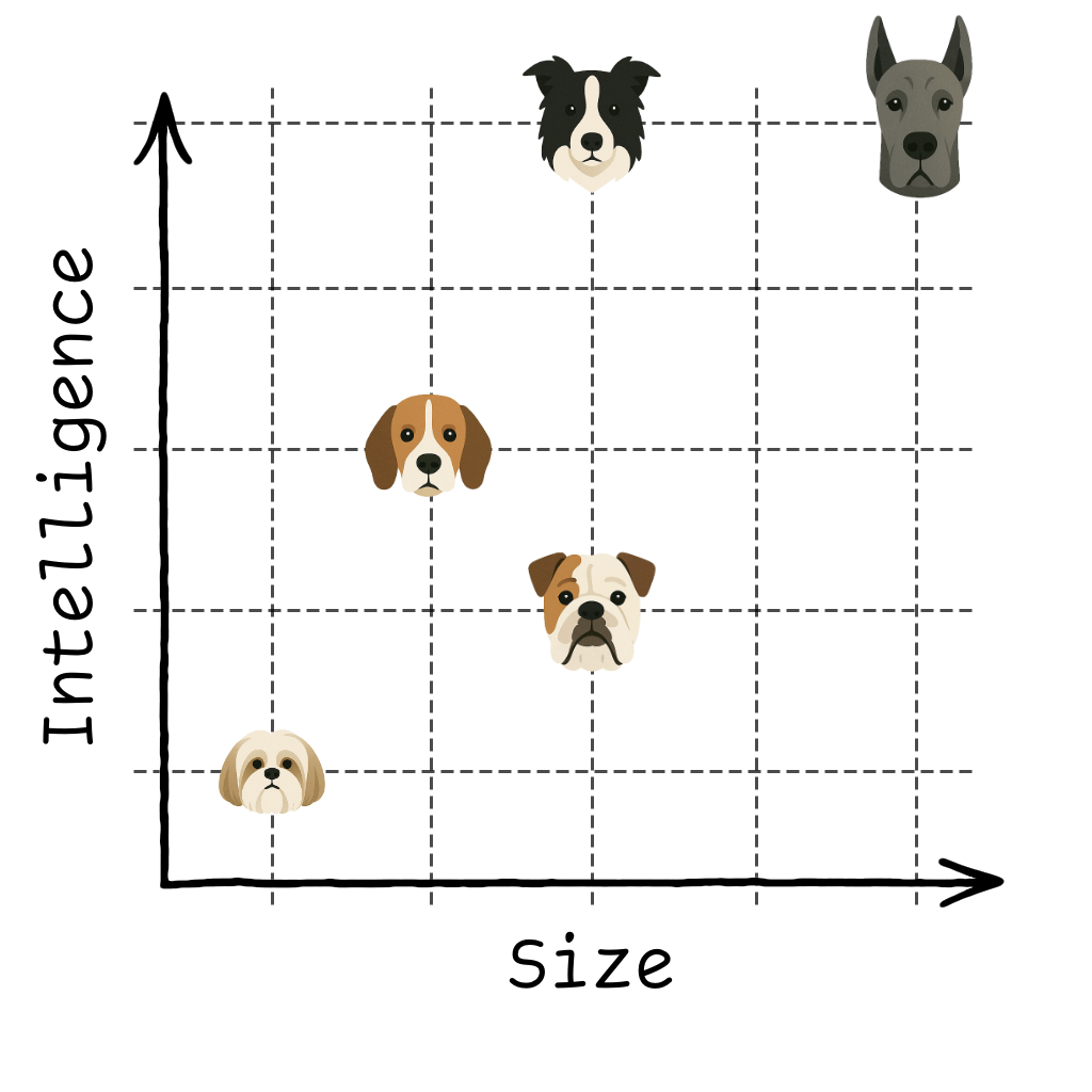
For each dog, we’ve defined a vector where the first column is size, and the second column is intelligence. A vector is a fancy name for a row of numbers. And in two dimensions, we can plot this really easily:

Let’s do some vector maths using Manhattan distance. A Great Dane ([5,5]) is 5 units away from a Beagle ([2,3]):

greatDane: [ 5 , 5 ]  (Size, Intelligence)
   beagle: [ 2 , 3 ]  (Size, Intelligence)
--------------------------
Size Difference:         | 5 - 2 | = 3
Intelligence Difference: | 5 - 3 | = 2
--------------------------
Manhattan Distance =       3 + 2 = 5

(we’re using Manhattan distance here because it’s simple, but you might well use Euclidean distance instead)

A vector can be both a specific point in our dog-embedding space, but it can also be a direction:

Direction	Δ Size	Δ Intelligence
“Smarter”	0	+1
“Smaller”	-1	0

What’s like a Bulldog ([3, 2]) but smaller ([-1, 0]) and smarter ([0, 1])?

  bulldog: [ 3, 2 ] +
  smaller: [-1, 0 ] +
  smarter: [ 0, 1 ] =

           [ 2, 3 ] -> a beagle!

Key point: if we start to plot things by their attributes, and we give each attribute a number, we can use simple maths to find items that are close together (clustering) and we can easily find items that differ from a starting point in a certain way.

AND WHAT’S MORE: this holds up over as many dimensions as we want to define, not just two:

Breed	Size	Intelligence	Fluff	Zip	Note
Great Dane	5	5	1	3	Big, smart, sleek
Shih Tzu	1	1	4	2	Mostly pretty
Border Collie	3	5	3	5	Clever and bouncy
Basset Hound	2	1	1	1	Stoner vibes
Samoyed	4	3	5	4	POWER BALL

We can do the same distance calculations again, even with more vectors:

   greatDane:   [ 5, 5, 1, 3 ]  (Size, Int, Fluff, Zip)
borderCollie:   [ 3, 5, 3, 5 ]  (Size, Int, Fluff, Zip)
--------------------------------------
Size Difference:         | 5 - 3 | = 2
Intelligence Difference: | 5 - 5 | = 0
Fluff Difference:        | 1 - 3 | = 2
Zip Difference:          | 3 - 5 | = 2
--------------------------------------
Manhattan Distance = 2 + 0 + 2 + 2 = 6

tldr; an embedding is a vector of numbers that describes something, and that you can use to cluster things by similarity

(vector databases, like Pinecone or pgvector, are simply databases that are fast at calculating the distance between vectors, and finding vectors that are close to other vectors)

Classifying books

Dogs are easy mode, because there’s a limited number of breeds and attributes. Also, coming up with attributes ourselves is hard work, and laziness is an inarguable virtue, so let’s see if we can make the computer do the work for us here.

If we wanted to classify books instead, we’d need to do something different. Let’s start by defining a table of every book, and every word in the English language, with the values being the occurrences of each word in the book:

Book	a	about	alchemy	animal	farm	gods	magic	pig	…
The Alchemist	5102	105	18	15	1	2	12	0	…
Alias Grace	6530	150	0	8	2	1	1	0	…
American Gods	7800	180	1	25	3	88	20	0	…
Animal Farm	2150	50	0	95	60	0	0	35	…

Table 1: Number of word occurrences in each book

Our vocabulary of words becomes our dimensions (or columns) and each book becomes a vector in those dimensions (rows). This is called a bag of words, a “bag” being the technical term for a mathematical object that counts the occurrences of things (but discards the order they’re in).

Bag of words was state of the art in approximately the 1950s for classification. There are lots of problems with this approach, and understanding those problems and how they’re solved starts to bring us closer to understanding embeddings!

Stories vs sagas

One problem with our Bag of Words is that we end up with values that are proportional to the size of books, which might mean that two very similar books are quite far apart, just because they’re of very different lengths. If George RR Martin rewrote Animal Farm, it might end up very far away from the Orwell original simply due to his overly-lax editorial staff.

There’s a particularly elegant solution to this in terms of determining how close two items are by measuring the difference in angles from the origin towards them (cosine similarity), BUT there’s also the highly effective and really simple solution of just dividing the count of each word by the length of the book (normalization):

Book Title	’a’ (%)	‘about’ (%)	‘alchemy’ (%)	‘animal’ (%)	‘farm’ (%)	‘gods’ (%)	‘magic’ (%)	‘pig’ (%)	Other Words (%)
The Alchemist	11.34	0.23	0.04	0.03	0.00	0.00	0.03	0.00	88.33
Alias Grace	4.35	0.10	0.00	0.01	0.00	0.00	0.00	0.00	95.54
American Gods	4.22	0.10	0.00	0.01	0.00	0.05	0.01	0.00	95.61
Animal Farm	7.17	0.17	0.00	0.32	0.20	0.00	0.00	0.12	92.02

Table 2: Distribution of word occurrences in each book

which gets us most of the way there without fancy maths or words like cosine.

Dull words

We’ve also got a problem here with our Bag of Words by a bunch of noise being introduced by words that are frequent but unspeakably dull, like “a”, “the”, and “of”. Different authors may lean more heavily on some than others (meaning their books are further apart in the dimensions of “of” and “a”), but that gives us absolutely no useful information about the meaning or content of what they’re writing about: what we care about is occurrences of words like dragon and android and lascivious.

We could maintain a list of dull words (often called “stop words”), and strip them out, but that’s fiddly, insufficiently lazy, and doesn’t account for the fact that what we consider to be a “stop word” might differ depending on the context.

Instead, we can use some simple statistics to look at how often a word (or “term”) appears in a given book/document compared to how frequently it appears across all of the books or documents we’re looking at; this is called “TF-IDF”, and it was state-of-the-art circa 1972:

TF-IDF(word, document, corpus) = TF(word, document) * IDF(word, corpus)

TF( word, document ) = literally the number of times the word appears in the document
IDF( word, corpus )  = how common or rare a word is across the entire collection of
                       documents -- it's *higher* for rare words, and *lower* for
                       common words

(you can see the actual formula and learn more about TF-IDF here)

KEY POINT: We’re still very firmly in a “words are dimensions, and books exist as points in that high-dimensional space” place here. We’re still representing books by a vector of numbers and looking for similarity by searching how close these books are to each other in a high-dimensional space. We’re just using a slightly fancier way of determining what those numbers should be.

Unsolvable problems

Our approach has gotten us some of the way towards classifying books well, but we start to hit some insurmountable problems in this approach:

• If we have a dimension for every word in English, we have waaay too many dimensions. One for each word, and each variation of each word. At least 50,000 if we’re just covering common English words. This starts to be cumbersome and computationally expensive to do maths on.

• Fantasy authors who insist on inventing spellings for “Sir”; there’s quite a lot of semantic information about a book embedded in having nobles with fancy titles prancing around, but our current approach gets confused when authors decide to start calling their characters “Ser” or “Syr” or “Sür” to try and sound more mysterious. More generally, we treat words with similar meanings but different spellings or forms as completely different dimensions

• Barking up the wrong tree: sometimes two different words are spelled identically (eg “bark”), and we don’t especially want to say that books on forestry and similar to books on puppies

• Word order is important! If your main character is a “dog who bites a bone” that’s likely quite a very different story from your “bone who bites a dog” character, even if the bone is haunted in both cases

tldr; vectors that are simply word frequency counts are a good start, but have a whole host of problems: we need something even smarter (embeddings) to do really good clustering and classification

Classifying words

We have until this point been thinking about how we would classify a whole book, and using word counts as dimensions. But what if we wanted to classify just one word instead?

If we were able to come up with vectors for individual words, we could start to address the problem that “dog”, “puppy”, and “pooch” are all treated as completely different things when classifying text, and we’d also get some other useful features, like it would make it easier for us to build things like fuzzy-search for users: “pooch pics” and “dog photos” should return much the same results when a user is searching for them.

We could hand-pick some dimensions to use for this:

Word	Concrete-ness	Happy	Is Living	Human-Related	Is Food
puppy	4	5	5	4	0
rock	5	3	0	1	0
love	1	5	0	5	0
sadness	1	1	0	5	0
run	2	2	0	4	0
computer	5	3	0	4	0
apple	5	4	5	3	5
democracy	1	4	0	5	0

This … might work pretty well with enough dimensions! But hand-choosing each of the dimensions we’d need and then manually classifying (and tweaking) 50,000 words feels like it might be a lot of hard work. Hard work that the computer should be doing for us… But how do we get the computer to do that for us? The computer would need to know already what the words meant in order to do the classification, so we need a way to bootstrap that process.

One intriguing idea might be to suck in a dictionary, and to use our bag-of-words techniques on the definition of each word to come up with a vector for each word. This however gives us our own bootstrapping problem: if we look at the dictionary definition for “puppy”, it’s very different for the one for “dog”: instead, it points us to the one for “dog” instead, and solving all of this starts to sound like complicated maths will be needed.

What if we instead tried to “know a word by the company it keeps”? It’s an idea that’s been floating around linguistics for decades, and suggests that words appearing in similar contexts probably have similar meanings. If you constantly see the words “dog” and “pooch” surrounded by words like “walk”, “leash”, “bark”, and “treats”, maybe you don’t need a dictionary to figure out they’re related?

Let’s game out how this could work: you could take every piece of written text you could lay your hands on, and go through it word by word, looking at the two words ahead of it and the two words behind it. For every word, you could start to build out the probability that any other word was in those four surrounding words.

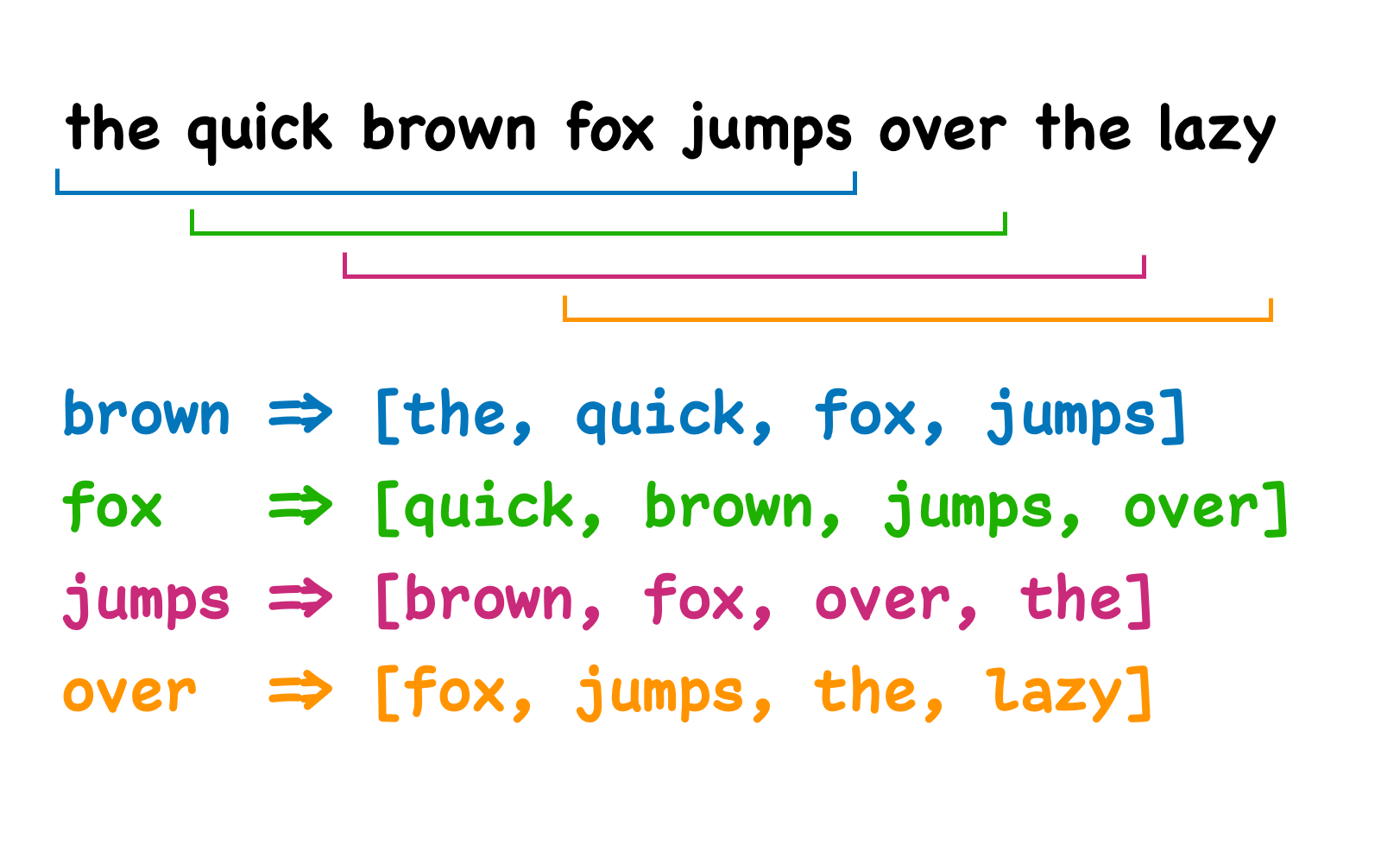
Figure 1: a sliding context window, associating each word in a sentence with the two words before and after it

You could use those probabilities as the values in your vector for each word, with every other word being a dimension still, and voila, you have per-word vectors that put “pupper”, “dog”, and “pooch” very close to each other.

This is almost the massive breakthrough that researchers at Google had in 2013 inventing “Word2Vec” (word to vector), but there’s one further, crucial refinement.

Dense Vectors

Our method above has two big problems. The first is one we’ve already identified: you still end up with an absolutely massive number of dimensions! These are unwieldy, difficult to work with, and computationally expensive to work with. But secondly, there’s just not enough reading text out there to make this work: there are infinite possible and sensible combinations of words, and while us humans have written down a lot of stuff, it turns out there’s simply not enough training data to make the above approach practical, IN ADDITION TO having all the drawbacks that come with these huge, unwieldy vectors.

So, when in doubt, make the computer do the work. And the tool that proved exceptionally useful for this is the mighty Neural Network.

A deep-dive into how they work is out of scope, even for this increasingly long article, but the key things to know are:

• They take vectors as their inputs and spit out vectors as their outputs

• They’re specialized tools for learning things through giving them examples

• They’re really good at prediction tasks

And so we can flip our earlier method on its head:

Rather than building a huge matrix of every word and its neighbours, how about we train a Neural Network to predict what a word is, based on some neighbours?

The process for this sounds like magic:

• We choose a number of dimensions we want to use, let’s say 300

• We literally just make up a 300-number-long vector for every input word: it’s literally just random to begin with

• We show the Neural Network billions of sets of four words, and ask it to guess the middle word

• We make tiny adjustments to each of those initial random vectors based on how well the Neural Network did at guessing it (using some complicated maths called “back-propagation”)

And over the billions and billions of times we do this, the computer eventually comes up with its own vectors for every word: vectors that really are good enough to predict what a word is going to be given its neighbours.

These same “guessing” vectors encode the meaning of words in a truly jaw-droppingly effective way. Again, it’s the principle that ‘a word is known by the company it keeps.’ If the network gets good at predicting surrounding words, the vectors it develops for each word must encode information about that word’s typical context, which relates closely to its meaning.

First of all, it puts related words close together. “Pupper”, “pooch”, and “doggo” now all sit really close together in our dimensional space. “Sir/Ser/Syr” basically sit on top of each other. We can’t really figure out what each of these dimensions means individually: there’s not a dedicated dimension for “dog like”, but they seem to work.

Secondly, remember how a vector can be either a point or a direction? Well it turns out if we start out at the vector for “king”, we subtract the vector for “man”, and add the vector for “woman”, we end up with a vector that’s almost identical to the one for “queen”. Complex semantic meaning has been encoded into our dimensions and embeddings. This shows the model learned abstract relationships (like gender and royalty) from the text data alone, encoding them into the vectors.

The above is the essence of “Word2Vec”.

Just a quick recap FAQ:

• Do we know why this works so well? NO

• Is this some bad-ass alien technology shit? YES

• Isn’t this a cause for alarm given how much we’re starting to rely on this technology and its successors? Please take your negativity out of the AI acceleration seminar

These dense vectors that capture semantic information along dimensions that the computer literally just made up are “embeddings”. These word embeddings can then be combined (using various methods, from simple averaging to more complex techniques) to create embeddings for sentences or even whole paragraphs: you have a long list of numbers that encodes the meaning of that sentence or that paragraph.

These dense vectors help solve our earlier problems: the fixed, lower dimensionality (e.g., 300) is manageable; words with similar meanings learned from context (like ‘Sir’ and ‘Ser’) end up close together; and the context-based learning helps differentiate meanings of words like ‘bark’ depending on surrounding words (though context handling gets even better later).

These paragraph-level embeddings are what underpin most RAG systems; in practice, people use the more clever versions of embeddings that the rest of the article covers, but still. An embedding is a row of numbers that describe the meaning of some words, and then we can use simple linear algebra to cluster related things together, or move around inside the vector space using abstract paths such as “positive sentiment” or “more feminine”

You can at this point leave the article, with a pretty good idea of what embeddings are. You won’t have learned how they deal with misspellings, words that are written the same and are completely different, or word ordering, BUT, you will know that it’s possible to encode semantic meaning into vectors of a few hundred numbers. Rather than leaving the article, you can also skip ahead to Part 3, which explains how embeddings are actually used in AI.

Classifying Sequences

With Word2vec, we end up with vectors that capture semantic meaning of words, and the vectors exist in a dimensional space that the computer learned by playing a guessing game over and over again. That the computer learned these dimensions by itself, and each dimension has a subtle and dense meaning means that we call those vectors “embeddings”.

We’ve also covered that you can average out these embedding to get a meaning for a sentence or a paragraph, but because this averaging process is treating those vectors as a “bag” (an unordered count of items), we lose a huge amount of meaning: the vectors for “man eats shark” and “shark eats man” are identical, even though the actual meanings differ substantially.

So rather than averaging our embeddings together, we need an operation that takes into account the sequence of the embeddings.

One of the first successful ways of doing this was with “Recurrent Neural Networks” (RNNs) – “recurrent” in this case means a neural network that accepts its last output as part of its next input (the state “recurs”). (there’s a little white lie here about the order in which these events happened that we’ll address later)

Here we start out with a base vector, and we imprint each vector in the sequence on it, one at a time. After we’ve stamped each vector representing a word onto the base vector, the base vector ends up changed in a way that reflects the sequence.

Here’s some Play-Doh as an example. The Play-Doh square is our base vector, and each stamp we apply over the top of the last one is the vector for a word. You’ll note that the order matters, and also that the most recent word vector ends up playing a larger role in the overall pattern we end up with than the previous ones.

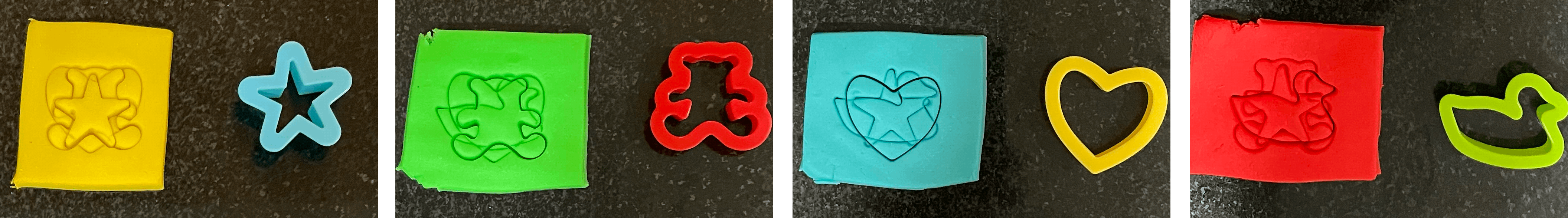
Figure 2: Pressing the same shapes into Play-Doh in different orders results in subtly different patterns, with the last shape often over-represented, and a faded initial shape

With Play-Doh, the more shapes you overlay on top of each other, the more you lose the previous shapes. If you add too many, you’ll end up with a complete mess you can’t make any sense of. This happens with actual Recurrent Neural Networks (RNNs) too! Despite this, it represented a significant improvement over just averaging together vectors.

Some clever mechanisms were invented to try and prevent earlier vectors getting completely wiped out by later ones, with fancy names like LSTMs and GRUs, but both represented incremental improvements over RNNs rather than a huge leap forward.

Historical note: the above describes events as if the sequence of events was: Word2Vec -> RNNs -> LSTMs and GRUs, which isn’t accurate! RNNs as a concept and LSTMs as a refinement of them actually predate Word2vec. So, what were they using as their input vectors before we got the rich “embeddings” that Word2vec gives us? They were either using the huge “one dimension per word” vectors we discussed near the beginning of the article, or were feeding in one character at a time with each character being a dimension. Using neural networks that can understand sequences rather than bags has all sorts of uses outside of text classification, but using the newly invented Word2vec “embeddings” with these techniques was a massive leap forward.

So at the end of this section, we have improved on our Word2Vec embeddings by building embeddings that combine other embeddings in the right sequence, which solves our problem of “man eats shark” / “shark eats man”. However, we have serious problems with losing information over sequences of any real length: by the time we get to the end of “the quick brown fox jumps over the lazy sheep dog”, we’ve added so much extra information that “quick” and “brown” have kind of been smushed together, and we’re very much more “dog” focused than we are “fox” focused because it occured later in the sentence.

Figure 3: After each addition of a vector onto our hidden state, previous vectors get “blurrier” and more recent vectors dominate

Attention, Transformers, Tokens

RNNs gave us much stronger embeddings than we had before, but ultimately these days we derive embeddings from the same technology that powers Large Language Models: a technique called attention and the system that uses it, the transformer. A proper deep-dive into the steps that take us from RNNs to transformers is too big for this already unwieldy article, but in short we train the computer to pay more attention to some words in a sentence than to others.

That’s probably how us humans do it too: your brain naturally ‘pays attention’ to the most important words (like the subject and verb, or key nouns) and how they relate, even if they are far apart. The ‘attention mechanism’ in AI tries to mimic this.

When processing a sequence of words, with attention we keep track of all the intermediate embeddings we’d generated rather than mashing them all together into one single vector. We add an extra neural network over that where we train further vectors to correlate how important each word is to every other word in the sequence. This whole system – including the new neural network – is trained the same way as we trained RNNs: by playing “guess the word” and getting the computer to update its internal parameters when it gets something right or wrong, until it’s usually getting them right!

Transformers take this attention mechanism even further, and are the technology that powers large language models. Using those to generate our embeddings, we get embeddings that can accurately describe even pretty long pieces of text well, and are free of almost all of the issues we’ve identified so far in this article. Commercial vendors like OpenAI offer very effective (and cost-effective!) general-purpose APIs for turning large chunks of text into embeddings for use in your applications.

Two things to clean up:

First of all, rather than using whole words as inputs, LLMs use tokens. These are fragments of words that are chosen (by the computer) during training to be a representative sample of commonly-appearing sequences. By using bits of words instead of whole words, we gain the ability to deal with words we haven’t seen before, which includes misspellings of words. For example, it might understand ‘embeddingtastic’ by recognizing the known tokens ‘embedding’ and ‘tastic’.

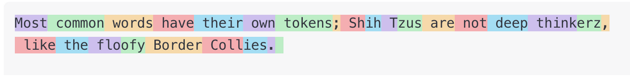
Figure 4: the OpenAI tokenizer in action. Common words are their own tokens, but less common words are split into fragments to help deal with the vast range of possible words including misspellings.

Secondly, chances are the majority of time you spend using LLMs you’ll be using “autoregressive” ones: they generate the next token for you, token by token. There are however important LLMs that are trained to guess the missing token inside a block of text, that will use the tokens both before and after the target token to try and figure it out: guess the word, but the word in the middle of the sentence instead of the next word.

Embeddings in the real world

OK, so we’ve learned what embeddings are, and they’re pretty darn cool, but why do we care? When are you, the busy young lady or young man, actually going to interact with an embedding? We hand-waved over it a little before, but the embeddings created using the same mechanism as LLMs (transformers) can take in very long pieces of text and give back exceptionally sophisticated vectors that capture complex meanings from that text. These aren’t just theoretical toys; they’re the mechanism behind a surprising amount of what we call AI today.

(we’ve also pretended that embeddings are just for working with text, which also isn’t true, but we’re already at over 5,000 words here…)

Classification

Remember classifying dogs? We picked the features: size, intelligence, fluffiness. Easy for dogs, but hopeless for text. Trying to hand-pick features for classifying emails or news articles (“Does it mention ‘invoice’?” “How many times does ‘politics’ appear?”) is fragile and labor-intensive. Embeddings flip this entirely. Instead of us telling the computer what features matter, the computer learns the important features itself when creating the embedding, using the guessing game we outlined above. These aren’t just keyword counts; they’re learned features capturing the underlying topic, the vibe, the subtle nuances.

Think about classifying customer reviews as ‘Positive’ or ‘Negative’. A simple keyword approach gets tripped up by sarcasm, varied phrasing, or subtleties in word ordering. Embeddings, however, capture the overall essence. They turn the review into coordinates in a high-dimensional ‘meaning space’. A happy review’s embedding might land near coordinates representing ‘joy’ and ‘satisfaction’ (dimensions the model learned!), while an angry one lands near ‘frustration’. The magic is that embeddings handle nuance: synonyms like “happy,” “pleased,” and “elated” end up in the same positive neighborhood.

So, you feed this rich embedding – these coordinates packed with learned features and context – into a classifier model. The classifier’s job becomes much simpler: it just learns to draw boundaries in that meaning space. “Everything landing in this region is Positive, everything over there is Negative.” The embedding does the heavy lifting of understanding the text; the classifier just reads the map. It’s spookily effective.

Clustering

Sometimes you don’t know in advance what categories you want to put things into. You’ve got a mountain of customer reviews, research papers, or social media posts, and you just want to know “what are the main themes here?” This is where clustering comes in, and embeddings super-charges it.

Because embeddings place texts with similar meanings close together in that high-dimensional space we keep talking about, we can use algorithms to automatically find groups, or “clusters,” of related items. Think back to our dogs: if we plotted thousands of individual dogs based only on their learned embeddings (without knowing breeds), clustering algorithms could find the clumps corresponding to Poodles or Beagles just by seeing which dogs’ vectors are close together.

It’s the same for text: these algorithms scan the positions (embeddings) of your documents in meaning-space and identify these natural groupings. Suddenly, you can see that your customer reviews naturally fall into clusters like “Complaints about Shipping”, “Praise for Product Quality”, and “Confused People Asking How To Turn It On”. No predefined categories needed, the structure just emerges from the meaning captured in the embeddings.

RAG (Retrieval-Augmented Generation)

This is the technique du jour for making LLMs smarter and more factual, and it leans heavily on embeddings. The core idea is surprisingly elegant: when you ask an LLM a question, you first use the embedding of your question to find relevant pieces of information (like paragraphs from a document) from a database.

How? Because of a slightly magical property: the embedding for a question is often geometrically close to the embedding of the text containing its answer within that vector space. It’s like the question “Where is the Eiffel Tower?” generates a vector that points towards the same region of meaning-space as the text “The Eiffel Tower is a wrought-iron lattice tower on the Champ de Mars in Paris, France.”

So, in a RAG system, you take the user’s query, generate the embedding for it, and then use a vector database (a fast database optimized for finding close vectors) to retrieve the chunks of text from your provided documents whose embeddings are closest. You then stuff these relevant chunks from your knowledge base into the prompt you give the LLM along with the original question. Voilà! The LLM now has the specific information needed to answer accurately, rather than just relying on its (potentially outdated or hallucinated) general knowledge. It’s like giving the LLM an open-book exam, using embeddings to find the right page in the textbook.

Autoregressive Generation

Okay, slight caveat here: the final output embeddings we’ve discussed (like the ones you get from OpenAI’s API) aren’t exactly what LLMs use second-by-second to generate text. But the underlying principle is deeply connected.

When an LLM is writing text, predicting the next token (word fragment), it maintains an internal “state.” This state is essentially a complex, evolving vector representation that captures the meaning and context of everything generated so far. Think of it as a temporary, super-sophisticated embedding of the preceding sequence. This internal state vector is what the LLM uses to figure out the probabilities for what the very next token should be.

So while you don’t directly use a final document embedding to generate text token-by-token, the same transformer architecture and attention mechanisms that create those powerful final embeddings are also at work inside the LLM, constantly creating and updating internal context vectors (which behave a lot like embeddings) to drive the generation process. It’s all part of the same family of vector-based meaning representation.

Conclusion

So, there you have it! Embeddings! Aren’t they cool?! We started with simple lists of numbers describing dogs, wrestled with the messy realities of counting words in books, and journeyed through decades of AI research, from Bag of Words to TF-IDF, Word2Vec, RNNs, and finally the mighty Transformers.

What we ended up with are these dense, powerful vectors – embeddings – that somehow manage to capture the meaning of text in a way that computers can work with mathematically, while just literally being lists of numbers. They’re not just lists of word counts; they’re rich representations learned by machines playing incredibly complex guessing games, encoding semantic relationships, context, and nuance along dimensions we didn’t even know we needed.

Are they slightly mysterious? Yes. Do we understand every nuance of why they work so well? Not entirely. But are they incredibly useful? Absolutely. From classifying spam, to finding themes in data, to making LLMs smarter with RAG, embeddings are a fundamental building block of modern AI. They might just be weirdly effective rows of numbers, but they’re our weirdly effective rows of numbers, and they’re changing how we interact with information. Thanks, embeddings.